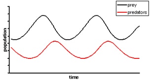
Life in the animal kingdom is a constant struggle for survival. Herbivores such as rabbits have to forage for food and breed avoiding carnivores that need to hunt and kill for their meals. This back-and-forth existence means that predators and their prey are locked in a cycle of population growth and contraction, which ecologists can model with mathematical equations.
 Infinite rabbits
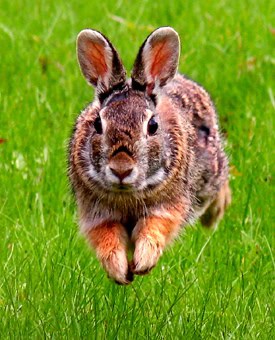
Imagine an island covered in grass and inhabited by a small population of rabbits. With no other animals around, the rabbits are free to eat and reproduce as they please. If you assume the number of rabbits that are born and die in a certain period is proportional to the total number of rabbits at that time, the change in their population is
dN/dt = rN.
Here N is the number of rabbits at time t, and r is the growth rate of the rabbit population, the difference between the birth and death rates.
Solving the differential equation gives
where N0 is the initial population of rabbits at time t = 0. The equation is an exponential function, which is why this model is often called the exponential growth model, and there are two possible outcomes. If there are more rabbit births than deaths, then the growth rate is positive and the population increase exponentially. If the opposite is true and the growth rate is negative, eventually there won’t be any rabbits left.
Limited options
The exponential model is easy to understand, but it’s not very realistic. With a positive birth rate and enough time, the rabbits will eventually cover the entire island – and even then they’ll still continue to grow forever! Obviously that won’t actually happen, because at some point the rabbits will run out of food and living space. The island has a carrying capacity, the maximum number of rabbits that it can support, and once this is reached their population will remain steady. We can add the concept of a carrying capacity K to the exponential growth model by adjusting the differential equation to become:
This equation is called the logistic model, and although finding its solution is more complicated than the exponential model, we can still get an idea of how it behaves by examining the relationship between N and K. When N is small, (K-N)/K is close to 1, so it doesn’t change the equation by much. As N gets closer to K however, (K-N)/K gets smaller, reducing dN/dt until it eventually hits zero and the rabbit population stops growing. If N is bigger than K, meaning the rabbit population is larger than the island can handle, (K-N)/K becomes negative and the population shrinks to a more manageable level. The exact behaviour of the model depends on the growth rate r, and for certain values the population level becomes chaotic, meaning it rapidly changes in a way that seems almost random.
 Unleash the foxes
The logistic model is a good description of a single animal population, but in real life the rabbits are unlikely to have a whole island to themselves. When even small areas of land can contain hundreds of different animals, modelling the interaction of an entire ecosystem is no easy task. A starting point is the predator-prey model, which describes the interaction between one species and it’s prey.
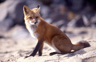
Imagine a small population of foxes is introduced to Rabbit Island. Now birth rate isn’t the only factor determining rabbit population, as some of them will be eaten by the foxes, who in turn will die if they don’t get enough food. The situation is described by the following equations, with x and y representing the rabbit and fox populations:
If there are no foxes around (i.e. y = 0), the first equation reduces to dx/dt=Ax, which is the simple exponential model. The additional term -Bxy represents rabbits being eaten by foxes, reducing the overall rabbit population. The second equation is a sort of mirror image of the first. Cxy represents the growth in fox numbers due to eating rabbits, and the negative growth rate -Dy means that without rabbits to eat, the foxes will quickly die off.
It’s not possible to get a general solution to this system of equations because they’re just too complicated. Instead, ecologists use computers to find numerical solutions, and plot graphs like the ones below:
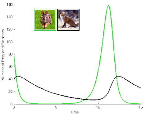
As you may remember from studying science at GCSE, predator-prey populations rise and fall in cycles. As the rabbit population increases there is more food for the foxes, so their population also increase. Eventually the foxes will be too many rabbits and their numbers will plunge. With a low rabbit population, foxes can’t get enough food and begin to die out, allowing the rabbit numbers to increase again and continuing the cycle.
A model existence
Whenever you make a mathematical model, you have to make a choice between accuracy and complexity. A simple equation like the exponential model is easy to solve but not very realistic, and the predator-prey model provides a more true to life picture but is harder to solve. Ecologists and mathematical biologists use advanced models to study natural habitats and learn more about the animal kingdom, and the same kind of maths describes the spread of infectious diseases. Understanding the natural world through maths helps us protect vulnerable species and appreciate their fight for survival.


